Spatial Data is stored in columns with the Geometry data type. The Geometry data type itself is an abstract (non-instantiable) class. It is the root class of the Geometry Type Hierarchy.
The geometry hierarchy is defined by the OGC document "OpenGIS Simple Features Specification for SQL". The following figure shows the hierarchy of the Geometry data type and its subtypes.
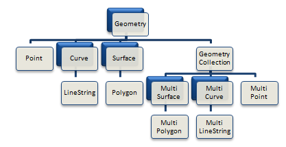
Not instantiable types in JASPA are highlighted in blue, these include Geometry, Curve, Surface, MultiSurface and MultiCurve. No constructor functions are defined for these types.
Seven members of the hierarchy are instantiable (Point, LineString, Polygon, GeometryCollection, MultiPoint, MultiLineString, and MultiPolygon). So, it is possible to create objects in these instantiable types.
The standard SQL-MM adds CircularString, CompoundCurve and CurvePolygon types. The new types extend the OGC geometry class hierarchy with circular arcs as curves and surfaces that have circular arcs as their boundary. JASPA doesn't support these new types, nonetheless PostGIS does in some functions.
A summary of the instantiable geometry subtypes and their descriptions is listed in the table below.
Table 5.1. Geometry Subtypes
| Geometry Subtype | Description |
|---|---|
| Point | A 0-dimensional geometry. It represents a single location in coordinate space. |
| LineString | A 1-dimensional geometry. It is a Curve with linear interpolation between points. |
| Polygon | A 2-dimensional geometry. It is defined by its exterior bounding ring and zero or more interior rings. |
| MultiPoint | A 0-dimensional geometry. It represents a collection of Points. |
| MultiLineString | A 1-dimensional geometry. It represents a collection of LineStrings. |
| MultiPolygon | A 2-dimensional geometry. It represents a collection of Polygons. |
| GeometryCollection | A 0, 1 or 2-dimensional geometry. It is a collection of one or more geometries. |
The OGC specification SFS 1.0 (1999) and SFS 1.1.0 (2005) were based on 2D geometries.
The SQL-MM specification extends the SFS spec by defining that features are in the two-dimensional coordinate space (x and y coordinates), and optionally they can have z and m coordinates. Z typically, but not necessarily, represent altitude. The M coordinate represents an arbitrary measurement.
The ST_CoordDim function return information about the dimension of a geometry.
The dimension of a Geometry object is less than or equal to the coordinate dimension. The possible values are:
- 0
Point and MultiPoint
- 1
LineString and MultiLineString.
- 2
Polygon and MultiPolygon.
The ST_Dimension function return information about the dimension of a geometry.
Establishing spatial relationships between geometric objects is a major objective of a GIS. Spatial relationships are based on the definitions of the interior, boundary, and exterior of a geometry. The concepts of interior, boundary and exterior are well defined in topology, and are also defined by the OGC “Simple Features for SQL”.
Interior
The interior of a geometry is the set of points that are left when the boundary points are removed.
Boundary
The boundary of a geometry is a set of geometries of the next lower dimension.
Exterior
The exterior of a geometry is the set of points not in the interior or boundary.
In the following table you can find the definition of the Interior, Boundary and Exterior for the different geometry types and also some examples.
| Geometry types | Interior | Boundary | Exterior |
|---|---|---|---|
| Point, MultiPoint | Point itself | Empty set | Points not on the interior or boundary of the geometry. |
| LineString | Set of Points that are left when the end points are removed. | Two End Points | Points not on the interior or boundary of the geometry. |
 |
 |
 |
Points not on the interior or boundary of the geometry. |
| LinearRing | All the LinearRing | Empty set | Points not on the interior or boundary of the geometry. |
 |
 |
Empty set | Points not on the interior or boundary of the geometry. |
| MultiLineString | Set of Points that are left when the boundary points are removed. | Those Points that are in the boundaries of an odd number of its element Curves | Points not on the interior or boundary of the geometry. |
 |
 |
 |
Points not on the interior or boundary of the geometry. |
 |
 |
 |
Points not on the interior or boundary of the geometry. |
| Polygon | Points within the Rings | The set of Rings | Points not on the interior or boundary of the geometry. |
 |
 |
 |
 |
| MultiPolygon | Points within the Rings | The set of Rings of its Polygons. | Points not on the interior or boundary of the geometry. |
 |
 |
 |
 |
In the definition of each function in the Chapter 9, Reference, you can find a table similar to the following one. It is used to indicate if the function supports 2D, 3D or measures.
Coordinate Dimensions
| 2D | 3D | M |
|---|---|---|
 | | |
![[Note]](images/note.png) | |
Although in the table we indicate 3D, it should be strictly called 2.5 D as z values are recorded as an attribute for each data vertex (x,y). |
In some functions even though we put a check mark in the 3D or M cell, the support depends on the configuration of the input geometries. The examples below, of ST_Union, try to illustrate it:
Example 1
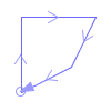
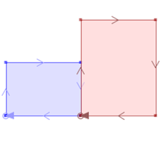
In the next example the union of two partially overlaid polygons creates two new vertex with height zero, while the preexistent ones keep their original heights.
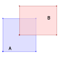 | 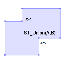 |
SELECT ST_AsEWKT(ST_Union(A,B)) from
(SELECT ST_GeomFromText('POLYGON ((40 20 1, 40 100 2, 120 100 3, 120 20 4, 40 20 5))',25830) as A,
ST_GeomFromText('POLYGON ((80 60 6, 80 130 7, 170 130 8, 170 60 9, 80 60 10))',25830) as B) as foo;

-Result
SRID=25830;POLYGON ((40 20 1, 40 100 2, 80 100 0, 80 130 7, 170 130 8, 170 60 9, 120 60 0, 120 20 4, 40 20 5))
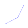
Example 2
In the next example the union doesn't create new vertexes. The vertexes of the new Polygon inherit the heights of the orginal vertexes. In case of a spatially common vertex, it would inherit the height of the vertex of either the polygons, it won't be interpolated.
 | 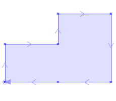 |
SELECT ST_AsEWKT(ST_Union(A,B)) from
(SELECT ST_GeomFromText('POLYGON ((20 10 2, 20 60 4, 90 60 6, 90 10 -2, 20 10 2))') as A,
ST_GeomFromText('POLYGON ((90 10 -2, 90 100 -4, 160 100 -6, 160 10 -8, 90 10 -2))') as B) as foo;

--Result
POLYGON ((20 10 2, 20 60 4, 90 60 6, 90 100 -4, 160 100 -6, 160 10 -8, 90 10 -2, 20 10 2))
Example 3
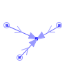
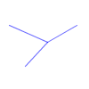
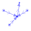
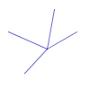
When an union of two consecutive lines is performed, the vertex height of the firtst line in the forward direction is assigned to the common vertex.
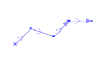 |
SELECT ST_AsEWKT(ST_Union(A,B)) from
(SELECT ST_GeomFromText('LINESTRING (20 10 2, 40 30 4, 70 20 6, 90 40 8)') as A,
ST_GeomFromText('LINESTRING (90 40 -5, 120 40 -10)') as B) as foo;

--Result
MULTILINESTRING ((20 10 2, 40 30 4, 70 20 6, 90 40 8), (90 40 8, 120 40 -10))The Dimensionally Extended- 9 Intersection Model (DE-9IM) is a mathematical approach to compare two geometries making pair-wise tests of the intersections between the Interiors, Boundaries and Exteriors of the two geometries, and finally it gives careful consideration to the dimension of the resulting intersections.
The DE-9IM, was developed by Clementini et al., which extends the 9 Intersection Model of Egenhofer and Herring.
A DE-9IM matrix has the form:
| B | |||
|---|---|---|---|
| A | Interior | Boundary | Exterior |
| Interior | dim( I(a) ∩ I(b) ) | dim( I(a) ∩ B(b) ) | dim( I(a) ∩ E(b) ) |
| Boundary | dim( B(a) ∩ I(b) ) | dim( B(a) ∩ B(b) ) | dim( B(a) ∩ E(b) ) |
| Exterior | dim( E(a) ∩ I(b) ) | dim( E(a) ∩ B(b) ) | dim( E(a) ∩ E(b) ) |
Each intersection can result in geometries of different dimensions. For instance, a intersection of two polygons can result in a point, a line, another polygon or an empty set. The term "dim(a)" represents the dimension of the geometries intersection as specified by ST_Dimension. The possible pattern values are:
- 0
An intersection must exist and its maximum dimension must be 0. (Point Intersection)
- 1
An intersection must exist and its maximum dimension must be 1. (Line Intersection)
- 2
An intersection must exist and its maximum dimension must be 2. (Area Intersection)
- T
An intersection must exist, the dimension doesn't care.
- F
An intersection must not exist. (Intersection is the empty set)
- *
It does not matter if an intersection exists or not.
The results returned by the DE-9IM are compared with a pattern matrix that represents the acceptable values for the DE-9IM.
The functions that test spatial relationships are:
Table 5.4. Spatial Relationships Functions
| Spatial Relationships Functions | DE-9IM pattern |
|---|---|
| ST_Contains | [T** *** FF*] |
| ST_ContainsProperly | [T** FF* FF*] |
| ST_Covers | [T** *** FF*] or [*T* *** FF*] or [*** T** FF*] or [*** *T* FF*] |
| ST_CoveredBy | [T*F **F ***] or [*TF **F ***] or [**F T*F ***] or [**F *TF ***] |
| ST_Crosses | [T*T *** ***] (for P/L, P/A, and L/A situations) [T** *** T**] (for L/P, L/A, and A/L situations) [0** *** ***] (for L/L situations) |
| ST_Disjoint | [FF* FF* ***] |
| ST_Equals | [T*F **F FF*] |
| ST_Intersects | [T** *** ***] or [*T* *** ***] or [*** T** ***] or [*** *T* ***] |
| ST_Overlaps | [T*T *** T**] (for P/P and A/A situations) [1*T *** T**] (for L/L situations) |
| ST_Touches | [FT* *** ***] or [F** T** ***] or [F** *T* ***] |
| ST_Within | [T*F **F ***] |
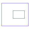
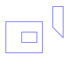
For example, the geometries of the following table have the intersection pattern matrix, [212 F11 FF2]. Therefore Geometry A Contains Geometry B, as they accomplish the ST_Contains pattern matrix [T** *** FF*].
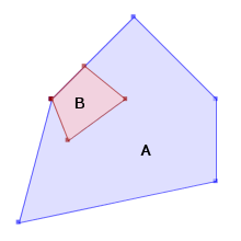 |
|
The ST_Relate function returns the DE-9IM pattern matrix of two geometries, or it tests the DE-9IM of those geometries correspond to a particular pattern matrix.
JASPA supports different types of formats for spatial data. WKB and WKT are defined in the OGC Simple Feature Access specification. EWKB and EWKT are PostGIS formats that add a SRID to WKB and WKT formats.
The Well-known Binary Representation for Geometry provides a portable representation of a geometric object as a contiguous stream of bytes.
You can use the ST_AsBinary function to convert geometries to their WKB representation. Inversely, ST_GeomFromWKB takes a WKB representation of a geometry and, optionally, a SRID as input parameters and returns the corresponding geometry.
binary WKB = ST_AsBinary(geometry);
geometry = ST_GeometryFromWKB(binary WKB, SRID);
geometry = ST_GeometryFromWKB(binary WKB);
The stream of bytes must be represented in a numeral system. PostgreSQL uses binary numeral system, whereas H2 uses hexadecimal representation.
SELECT ST_GeomfromText('POINT(0 0)');

--Result PostgreSQL:
\011 \000\001\000\000\000\000\000\000\000\000\000\000\000\000\000\000\000\000

--Result H2:
0920000100000000000000000000000000000000
Alternatively, you can use the function ST_AsHEXEWKB to obtain a geometry WKB representation in hexadecimal in both databases.
SELECT ST_AsHEXEWKB(ST_GeomFromText('POINT(1 1 1)',25830));
--Result PostgreSQL & H2:
01010000A0E6640000000000000000F03F000000000000F03F000000000000F03F

SELECT ST_AsText('01010000A0E6640000000000000000F03F000000000000F03F000000000000F03F');
--Result
POINT (1 1 1)The Well-known Text Representation of Spatial Reference Systems provides a standard textual representation for spatial reference system information.
| Geometry Type | Example | Comment |
|---|---|---|
| Point | POINT (0 0 10) | Point with Z coordinate |
| LineString | LINESTRING (1 1 2 5, 2 1 4 8, 2 2 6 10) | LineString with Z and M coordinates |
| Polygon | POLYGON ((1 1, 1 3, 3 3, 3 1, 1 1)) | Polygon |
| MultiPoint | MULTIPOINT ((0 0), (1 1))or MULTIPOINT (0 0, 1 1) | MultiPoint |
| MultiLineString | MULTILINESTRING ((1 1, 2 1, 2 2), (2 3, 3 3, 3 2)) | MultiLineString |
| MultiPolygon | MULTIPOLYGON (((1 1, 1 3, 3 3, 3 1, 1 1), (1.5 2, 2 2.5, 2.5 2, 1.5 2)), ((4 3, 4 5, 6 5, 6 3, 4 3))) | MultiPolygon, first polygon with a hole |
| GeometryCollection | GEOMETRYCOLLECTION (POINT (1 1), LINESTRING (1 3, 2 2, 2 1)) | GeometryCollection composed of a Point and a LineString. |
You can use the ST_AsText function to convert geometries to their WKT representation. Inversely, ST_GeomFromText takes a WKT representation of a geometry and, optionally, a SRID as input parameters and returns the corresponding geometry.
text WKT = ST_AsText(geometry);
geometry = ST_GeomFromText(text WKT);
geometry = ST_GeomFromText(text WKT, SRID);
Extended Well-known Binary. This format embeds the SRID to the geometry.
You can use the ST_AsEWKB function to convert geometries to their EWKB representation. Inversely, ST_GeomFromEWKB takes a EWKB representation of a geometry and returns the corresponding geometry.
binary EWKB = ST_AsEWKB(geometry);
geometry = ST_GeomFromEWKB(binary EWKB);
Extended Well-known Text Representation. This format embeds the SRID to the geometry.
You can use the ST_AsEWKT function to convert geometries to their EWKT representation. Inversely, ST_GeomFromEWKT takes a EWKT representation of a geometry and returns the corresponding geometry.
text EWKT = ST_AsEWKT(geometry);
geometry = ST_GeomFromEWKT(text EWKT);
Example
SRID=25830;POINT(719626 4369131 56.2)
The Geography Markup Language (GML) is the XML grammar defined by the OGC to express geographical features. GML serves as a modeling language for geographic systems as well as an open interchange format for geographic transactions on the Internet. JASPA supports OGC GML standard 2.1.2.
OGC GML standards can be found in http://www.opengeospatial.org/standards/gml
You can use the ST_AsGML function to convert geometries to their GML representation. Inversely, ST_GeomFromGML takes a GML representation of a geometry and returns the corresponding geometry.
text GML = ST_AsGML(geometry);
geometry = ST_GeomFromGML(text GML);
Example
<gml:Point>
<gml:coordinates> 1.0,1.0,1.0 </gml:coordinates>
</gml:Point>
Keyhole Markup Language (KML) is an XML language focused on geographic visualization. KML was developed for use with Google Earth. In 2008 KML Version 2.2 has been adopted as an OGC implementation standard, which can be found in http://www.opengeospatial.org/standards/kml/
KML uses 3D geographic coordinates: longitude, latitude and altitude. The longitude, latitude components are defined in WGS84.
You can use the ST_AsKML function to convert geometries to their KML representation. Inversely, ST_GeomFromKML takes a KML representation of a geometry and returns the corresponding geometry.
text KML = ST_AsKML(geometry);
geometry = ST_GeomFromKML(text KML);
Example
<kml:Polygon xmlns:kml="http://earth.google.com/kml/2.1">
 <kml:outerBoundaryIs>
  <kml:LinearRing>
   <kml:coordinates>
   -5.850379847879675,43.35970362178223
   -5.848336797975651,43.36161117272741
   -5.850411866073801,43.36311451294508
   -5.853216861450062,43.36175621008758
   -5.850379847879675,43.35970362178223
   </kml:coordinates>
  </kml:LinearRing>
 </kml:outerBoundaryIs>
</kml:Polygon>
A spatial database has associated metadata tables for describing the existence and properties of geometry columns. Each geometry column will be represented as a row in the GEOMETRY_COLUMNS metadata table. At the same time, every geometry column has associated a Spatial Reference System from the SPATIAL_REF_SYS metadata table.
| |
There is an auxiliary table _AVAILABLESRIDS for JASPA internal use which must not be deleted or manually edited. |
The GEOMETRY_COLUMNS table consists of a row for each geometry column in the database. The columns of this table are:
Table 5.6. GEOMETRY_COLUMNS table
| FIELD | TYPE | NULL | KEY | DEFAULT |
|---|---|---|---|---|
| F_TABLE_CATALOG | VARCHAR(256) | NO | PRIMARY | NULL |
| F_TABLE_SCHEMA | VARCHAR(256) | NO | PRIMARY | NULL |
| F_TABLE_NAME | VARCHAR(256) | NO | PRIMARY | NULL |
| F_GEOMETRY_COLUMN | VARCHAR(256) | NO | PRIMARY | NULL |
| COORD_DIMENSION | INTEGER(10) | NO | NULL | |
| SRID | INTEGER(10) | NO | NULL | |
| TYPE | VARCHAR(30) | NO | NULL |
F_TABLE_CATALOG, F_TABLE_SCHEMA, F_TABLE_NAME
The fully qualified name of the feature table containing the geometry column. F_Table_Catalog field is unused in JASPA.
F_GEOMETRY_COLUMN
The name of the column in the feature table that is the geometry column.
COORD_DIMENSION
Code for the coordinate dimension. The coordinate_dimension must be an integer (2 for XY coordinates, 3 for XYZ or 4 for XYZM).
SRID
The ID of the spatial reference system used for the coordinate geometry in this table. It is a foreign key reference to the SPATIAL_REF_SYS table.
TYPE
The type must be an uppercase string corresponding to the geometry type (e.g, MULTIPOLYGON,LINESTRING).
The SPATIAL_REF_SYS view stores information on each Spatial Reference System (SRS) in the database. It is pre-populated with SRS and EPSG values. The columns of this table are:
Table 5.7. SPATIAL_REF_SYS view
| FIELD | TYPE | KEY | DEFAULT |
|---|---|---|---|
| SRID | INTEGER(10) | NULL | |
| AUTH_NAME | VARCHAR(4) | NULL | |
| AUTH_SRID | INTEGER(10) | NULL | |
| SRTEXT | VARCHAR | NULL |
SRID
Spatial Reference System Identifier. It constitutes a unique integer key for a Spatial Reference System within a database.
AUTH_NAME
Spatial Reference System Authority Name
AUTH_SRID
Authority Specific Spatial Reference System Identifier
SRTEXT
Well-known Text description of the Spatial Reference System
A spatial reference system, also referred to as a coordinate system, is a geographic (latitude-longitude), a projected (X,Y), or a geocentric (X,Y,Z) coordinate system.
The well-known text representation of spatial reference systems provides a standard textual representation for spatial reference system information. The definition for the string representation of a coordinate system is as follows:
<coordinate system> = <projected cs> | <geographic cs> | <geocentric cs>
<projected cs> = PROJCS[‘<name>‘, <geographic cs>, <projection>, {<parameter>,}* <linear unit>]
<projection> = PROJECTION[‘<name>‘]
<parameter> = PARAMETER[‘<name>‘, <value>]
<value> = <number>
This WKT representation of an Spatial Reference System can be found in the SRTEXT column of the SPATIAL_REF_SYS view. As an example, geographic WGS84 is defined as:
| SRID | AUTH_NAME | AUTH_SRID | SRTEXT |
|---|---|---|---|
| 4326 | EPSG | 4326 | GEOGCS["WGS 84", DATUM["World Geodetic System 1984", SPHEROID["WGS 84", 6378137.0, 298.257223563, AUTHORITY["EPSG","7030"]], AUTHORITY["EPSG","6326"]], PRIMEM["Greenwich", 0.0, AUTHORITY["EPSG","8901"]], UNIT["degree", 0.017453292519943295], AXIS["Geodetic latitude", NORTH], AXIS["Geodetic longitude", EAST], AUTHORITY["EPSG","4326"]] |
EPSG codes and their WKT representation can be found in http://spatialreference.org/
The function ST_Transform is used to transform a Geometry to a specified spatial reference system. This reprojection is done by means of the GeoTools library.
The GeoTools library is used to provide coordinate reprojection support within JASPA. It is done by the EPSG WKT Plugin which stores the SRS definitions in a Java properties file. The EPSG Geodetic Parameter Dataset is a structured dataset of Coordinate Reference Systems and transformations.
Transformation between coordinate systems can be carried out by equation-based methods or by grid-based methods:
Equation-based methods include Seven-parameter or Molodensky. A coordinate transformation can require and use the parameters of the Ellipsoids associated with the source and target coordinate reference systems, in addition to the parameters explicitly associated with the transformation.
Grid-based methods allow you to model the differences between the Coordinate Reference Systems and are potentially the most accurate method.
National Transformation version 2 (NTv2)
The NTv2 method uses a binary distortion Grid File to transform coordinates from one spatial reference system to another. This method is used for accurate datum shifts, instead of using coordinate transformations by parameters. GeoTools does not support NTv2, for this reason JASPA doesn't support it either.
GeoTools is also used for the JASPA shp loader in order to read .prj files from shapefiles. For further information about GeoTools, refer to http://www.geotools.org/
Queries on tables with many registers can be slowed down. To improve performance, it is advisable to create an index for your most queried fields, and besides it may be necessary to create spatial indexes.
An index allows the database server to find and retrieve specific rows much faster than it could do without an index. Without an index, when a table is queried, the system access to each table row sequentially. An index has disadvantages as well. First, every index increases the amount of storage used, and second, the index must be updated when the data are altered.
PostgreSQL 8.4 supports 4 index types: B-tree, Hash, GiST and GIN.
GiST index (Generalized Search Trees) is the most suitable index for querying spatial data. This operator classes two-dimensional geometric data as overlapping, or as inside or as at one side.
JASPA for PostgreSQL make use of GiST indexes combined with minimum bounding rectangles (also known as bounding boxes) of the geometries. The use of bounding boxes is commonly called R-tree index.
![[Warning]](images/warning.png) | |
Please note that JASPA for H2 database currently doesn't support spatial indexes. This section refers only to PostgreSQL database. |
To create an index use the CREATE INDEX command.
CREATE INDEX <index_name> ON <table_name> USING GIST (ST_PGBOX(<geometry_column_name>));
To remove an index, use the DROP INDEX command.
DROP INDEX <index_name>;
Indexes can be added to and removed from tables at any time. Once an index is created, it is advisable running VACCUM ANALIZE command to rebuild table statistics and calculate the maximum and minimum values. After this, no further intervention is required: the system will update the index when the table is modified.
VACUUM ANALYZE [table_name] ([geometry_column_name]);
The following is an example of creating an index, updating statistics and dropping the index.
CREATE TABLE myspatialtable (id serial);
SELECT AddGeometryColumn ('myspatialtable','geom',4326,'POINT',3);

Table myspatialtable

 Column |  Type   |
--------+---------|
 id     | integer |
 geom   | bytea   |

CREATE INDEX myspatialtable_geom_idx ON myspatialtable USING GIST (ST_PGBOX(geom));
VACUUM ANALYZE myspatialtable(geom);
DROP INDEX myspatialtable_geom_idx; | |
If the name of the geometry column is in upper-case you must call that column with double quotation marks, as shown in the following example: CREATE TABLE myspatialtable (id serial);
SELECT AddGeometryColumn ('myspatialtable','Geom',4326,'POINT',3);
CREATE INDEX myspatialtable_geom_idx ON myspatialtable USING GIST (ST_PGBOX("Geom")); |
Spatial indexes are used in spatial relationships queries. Once the index is built, the system uses it automatically. To avoid index use, call the functions using the prefix _. In particular JASPA use spatial indexes in the following functions:
Table 5.8. Functions using spatial indexes
| Functions using spatial indexes | Functions not using indexes |
|---|---|
| ST_Contains | _ST_Contains |
| ST_ContainsProperly | _ST_ContainsProperly |
| ST_Covers | _ST_Covers |
| ST_CoveredBy | _ST_CoveredBy |
| ST_Crosses | _ST_Crosses |
| ST_DWithin | _ST_DWithin |
| ST_Intersect | _ST_Intersect |
| ST_Intersects | _ST_Intersects |
| ST_Overlaps | _ST_Overlaps |
| ST_Touches | _ST_Touches |
| ST_Within | _ST_Within |
PostgreSQL includes automatically GiST indexes for these spatial operators:
Table 5.9. Spatial operators
| Operators | Meaning |
|---|---|
| << | Is strictly left of? |
| &< | Does not extend to the right of? |
| &> | Does not extend to the left of? |
| >> | Is strictly right of? |
| <<| | Is strictly left of? |
| &<| | Does not extend above? |
| |&> | Does not extend below? |
| |>> | Is strictly above? |
| @> | Contains? |
| <@ | Contained in or on? |
| ~= | Same as? |
| && | Overlaps? |
The following query would use a spatial index (if it had been created before)
--Find all restaurants within 1 kilometer of the hotels
SELECT r.name,h.name FROM restaurant as r,hotel as h WHERE ST_DWithin(r.geom,h.geom,1000);
To avoid the index usage:
SELECT r.name,h.name FROM restaurant as r,hotel as h WHERE _ST_DWithin(r.geom,h.geom,1000);
There are a large number of software products that could use JASPA as spatial database.
Any help to develop the JASPA connectors to other third party software will be appreciated. Specially we stand out connectors to servers (Geoserver...), GIS software programs (gvSIG, Quantum GIS, Kosmo, uDig ...) or GIS tools (GeoTools, OGR...).
Libpq is the C application programmer's interface to PostgreSQL. It is a set of library functions that allow client programs to pass queries to the PostgreSQL backend server and to receive the results of these queries.
Mapserver accesses to JASPA for PostgreSQL data using libpq and SQL sentences which are supported by JASPA thanks to its high level of Postgis compatibility.
http://mapserver.org/input/vector/postgis.html
Configure MapServer
The CONNECTION parameter is used to specify the parameters to connect to the database. CONNECTION parameters can be in any order. Most are optional. The CONNECTIONTYPE parameter must be set to POSTGIS, dbname is required, user is required, host defaults to localhost, port defaults to 5432 (the standard port for PostgreSQL).
The DATA parameter is used to specify the data used to draw the map.
DATA [geometry_column] FROM [table_name|sql_subquery] USING UNIQUE [unique_key] USING srid=[spatial_reference_id]
The “using unique” and “using srid=” clauses are optional, but using them improves performance.
CONNECTIONTYPE POSTGIS
CONNECTION "host=yourhostname dbname=yourdatabasename user=yourdbusername password=yourdbpassword port=yourpgport"
DATA "geometrycolumn from yourtablename using gid"
Mapfile example
LAYER
    NAME        "soils"
    CONNECTIONTYPE postgis
    CONNECTION "user=postgres password=postgrespg dbname=tutorial host=localhost"
    DATA        "geom from soils using unique gid"
    STATUS      ON
    TYPE        POLYGON
    GROUP       CARTOINICIAL

    FILTER "area(geom) > 10000 and soil_code >= 1"

    CLASS
      NAME            "Disponibilidad optima"
      EXPRESSION      ([soil_code] = 3)
      COLOR           164 164 164
      OUTLINECOLOR    255 255 255
    END

    CLASS
      NAME            "Disponibilidad menor"
      EXPRESSION      ([soil_code] = 1 or [soil_code] = 2)
      COLOR           192 192 192
      OUTLINECOLOR    255 255 255
    END
END
Mapserver uses the && operator to limit the search of geometries to a smaller area. Mapserver sends a query to JASPA similar to this one:
SELECT
 asbinary(force_collection(force_2d(geom)),'NDR'), gid::text
FROM suelos
WHERE geom && setSRID('BOX3D(4000 4500, 6100 7250)'::BOX3D,
find_srid('','soils','geom') )' 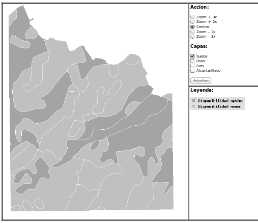 |
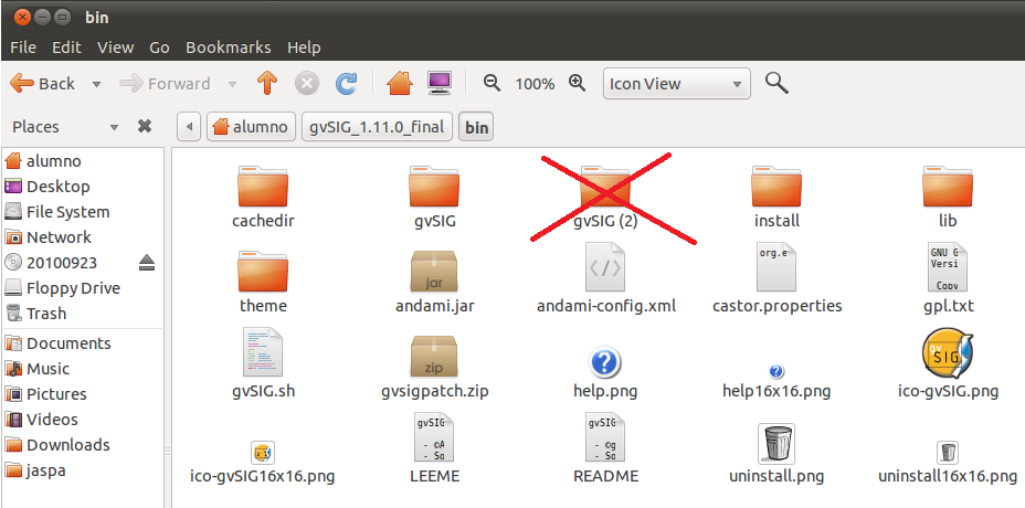
Enable Jaspa for gvSIG 1.11:
Copy the patch file "gvsigpatch.zip" into the bin directory of gvSIG installation. -> ... / .../gvsiginstallation/bin
Unpack in same directory. Overwrite if it asks.
| |
Check that when the gvsigpatch.zip is descompressed, it does not create any folder as gvSIG(2). |
To connect to Jaspa, we must choose as Driver: "PostGIS JDBC Driver": 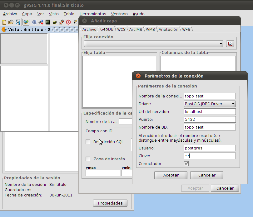 |
| |
gvSIG does not support editing simple geometries like LineString, Points or Polygons. |