This chapter provides a tutorial introduction to JASPA. We assume that JASPA is already installed on your machine, if it is not true refer to Chapter 3, Installation.
This chapter describes how to create the database and the tables needed, how to enter spatial data and some examples using the spatial data.
In order to complete the section Section 5, “Exercises” you should get these sql files located in the folder /doc/data of the JASPA distribution:
H2:
soilsh2.sql,usesh2.sql,riversh2.sqlPostgreSQL:
soilspg.sql,usespg.sql,riverspg.sql
The database can be created with the SQL command createdb on the command line:
shell> createdb -U <username> <database_name>The following step is to add the JASPA functionality. It can be avoided if you choose a JASPA template when you create your new database.
shell> createdb -U <username> -T <jaspa_template> <database_name>However if you are trying to spatially enable an existing database or you didn't have a JASPA template, you should follow these steps:
Install PL/Java
Windows
shell> psql -U <username> -f C:\jaspa4pg\sql\pljavainstall.sql -d <database_name>Linux
shell> psql -U <username> -f /opt/jaspa4pg/sql/pljavainstall.sql -d <database_name>Load the jaspa.sql file
Windows
shell> psql -U <username> -f C:\jaspa4pg\sql\jaspa.sql -d <database_name>Linux
shell> psql -U <username> -f /opt/jaspa4pg/sql/jaspa.sql -d <database_name>
Accessing to a Database
In order to connect to your database you can run the PostgreSQL interactive terminal program, psql, which allows you to execute SQL commands. Alternatively you can use an existing graphical frontend tool like pgAdmin.
shell> psql -U <user> <database_name>To obtain information about the JASPA installed version, you can use the following SQL sentences:
database=# SELECT Jaspa_Full_Version();

database=# SELECT Jaspa_build_date();
Remove an existing PostgreSQL database
You can remove the database simply with:
shell> dropdb [option...] <database_name>The first step consist of starting the H2 server. Open a command shell and run this command:
shell> h2The following command will automatically create a new, empty database if it does not exist. The database will be called myfirstjaspadb.
Windows
shell> h2runscript -url jdbc:h2:tcp://localhost/~/myfirstjaspadb -user sa -password 123 -script c:\jaspa4h2\sql\jaspa.sql -showResults
Linux
shell> h2runscript -url jdbc:h2:tcp://localhost/~/myfirstjaspadb -user sa -password 123 -script /opt/jaspa4h2/sql/jaspa.sql -showResults
Connecting to a database
In order to connect to your database you can use the H2 client (a browser). Open a command prompt shell and run the following command:
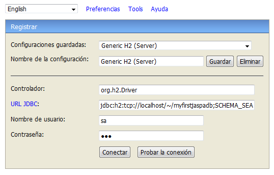
shell> h2consoleA browser window should open, enter there the connection parameters: database URL, user name, password.
| Parameter | Value |
|---|---|
| Saved settings | Generic H2 (Server) |
| Setting name | Generic H2 (Server) |
| Driver Class | org.h2.Driver |
| JDBC URL | jdbc:h2:tcp://localhost/~/<database_name>;SCHEMA_SEARCH_PATH=PUBLIC,JASPA |
| User Name | sa |
| Password | 123 |
Start the H2 server
shell> h2
Create the database tutorial
Windows
shell> h2runscript -url jdbc:h2:tcp://localhost/~/tutorial -user sa -password 123 -script c:\jaspa4h2\sql\jaspa.sql -showResults
Linux
shell> h2runscript -url jdbc:h2:tcp://localhost/~/tutorial -user sa -password 123 -script /opt/jaspa4h2/sql/jaspa.sql -showResults
Creating a table using SQL is quite easy. You just need the command CREATE TABLE. If the tables will store spatial data, then you need to use the JASPA function AddGeometryColumn.
Though it seems to be rapid, the design of the structure of the database (tables, columns, constraints, relationships...) is an important phase and can take a long time.
The first step is to create a normal table:
database=# CREATE TABLE <table_name> (<column_name> <data_type> <column_constraint> ... );
The next step is to add a spatial column to an existing feature table.
database=# SELECT AddGeometryColumn(<schema>, <table>, <column>, <srid>, <type>, <coordinate_dimension>);
To show the tables in the current database use the PostgreSQL command:
database=# \dt
Here is an example
database=# CREATE TABLE hospitals (
                        code integer PRIMARY KEY,
                        name varchar);

database=# SELECT AddGeometryColumn('public','hospitals', 'geom', 25830, 'MULTIPOLYGON', 2 );The first step is to create a normal table:
CREATE TABLE <table_name> (<column_name> <data_type> <column_constraint> ... );
The next step is to add a spatial column to an existing feature table.
SELECT AddGeometryColumn(<schema>, <table>, <column>, <srid>, <type>, <coordinate_dimension>);
Here is an example
CREATE TABLE hospitals (
 code integer PRIMARY KEY,
 name varchar);

SELECT AddGeometryColumn('PUBLIC','HOSPITALS', 'GEOM', 25830, 'MULTIPOLYGON', 2 );
Show the tables in the current database
SHOW TABLES;
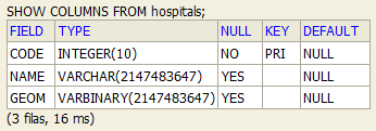
Display information about the columns in a given table:
SHOW COLUMNS FROM hospitals;
After you create your tables, you need to populate data into them. You can insert rows of data typing manually SQL statements or loading a SQL file.
INSERT INTO statement allows you to insert new rows into an existing table. The data inserted in the geometry columns must be a geometry representation. To build spatial values you can use Well-Known Text functions (i.e. ST_GeomFromText, ST_LineFromText) or Well-Known Binary functions (i.e ST_GeomFromWKB, ST_MPointFromText) or JASPA functions (i.e ST_MakePolygon, ST_MakePoint).
The following example uses the ST_GeomFromText function to insert a MultiPolygon.
INSERT INTO hospitals VALUES (10, 'A', ST_GeomFromEWKT('SRID=25830;MULTIPOLYGON (((20 20, 50 20, 50 50, 20 50, 20 20)))'));shp2jaspapg and shp2jaspah2 are two data converters that can be used to convert ESRI Shape files into SQL suitable for JASPA.
shp2jaspapg /// shp2jaspah2
java Converter [<options>] <shapefile> [<schema>.]<table>
The options of the shp converters are:
- -s <SRID>
Set the SRID field. If it is not specified then try to look for the .prj file. If the .prj does not exists uses -1.
- (-d|a|c|p) These are mutually exclusive options:
- -d
Drops the table, then recreates it and populates it with current shape file data.
- -a
Appends shape file into current table, must be exactly the same table schema.
- -c
Creates a new table and populates it, this is the default if you do not specify any options.
- -p
Prepare mode, only creates the table.
- -g <geocolumn>
Specify the name of the geometry column
- -k
Keep shape file column names case.
- -i
Use int4 type for all integer dbf fields.
- -info
Print some summarizing information about null geometries, not valid geometries, etc
- -I
Create a spatial index on the geocolumn.
- -S
Generate simple geometries instead of MULTI geometries. If a geometry contains 2 or more geometries then takes the first one
- -f
Fix invalid geometries according to the OGC. Clean and rebuild invalid POLYGONS or MULTIPOLYGONS.
- -w
Output WKT format. This option guarantee OGC compatibility. Note that this will introduce coordinate drifts
- -W <encoding>
Specify the character encoding of Shape's attribute column. (default : "ISO-8859-1") You can find a complete list of supported charsets in http://www.iana.org/assignments/character-sets
- -N <policy>
NULL geometries handling policy (insert|skip|abort)
- -n
Only import DBF file.
- -co <columnname>
Column to be included in the convertion.
- -CO <columnname>
Column to be excluded in the convertion.
- -?
Display the help screen.
Notes:
The table and geom column names are case sensitive
In PostgreSQL the default behaviour is to use lowecase
In H2 the default behaviour is to use uppercase
Type conversion matching:
DBF type precision(p) scale(s) Jaspa SQL type
Integer 0 < p <= 4 (length - 1) s = 0 SMALL INT
Integer 4 < p <= 9 (length - 1) s = 0 INTEGER
Integer 9 < p <= 18 (length - 1) s = 0 BIGINT
Integer p > 18 (length - 1) s = 0 NUMERIC (p, 0)
Real 0 < p <= 7 (length - 2) s > 0 REAL
Real 7 < p <= 14 (length - 2) s > 0 DOUBLE PRECISION
Real p > 14 (length - 2) s > 0 NUMERIC (p*2,p)
String length (length < 254) VARCHAR (length)
note: empty strings are considered null
Boolean BOOLEAN
Date DATE
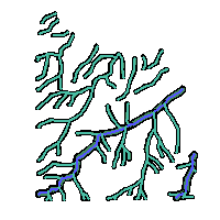
A shape file must be specifiedThe shp converter would create SQL sentences like these:
CREATE TABLE "rivers" ("GID" IDENTITY PRIMARY KEY, "river_code" INTEGER);
SELECT addgeometrycolumn ('rivers', 'geom', -1, 'MULTILINESTRING', 2);
INSERT INTO "rivers" ("geom", "river_code") VALUES (ST_GeomFromText ('MULTILINESTRING ((4260 7084, 4131 7030, 4078 6965))', -1), 2);
INSERT INTO "rivers" ("geom", "river_code") VALUES (ST_GeomFromText ('MULTILINESTRING ((4284 7001, 4217 6934, 4168 6860, 4058 6820))', -1), 2);
INSERT INTO "rivers" ("geom", "river_code") VALUES (ST_GeomFromText ('MULTILINESTRING ((4425 6833, 4375 6805, 4334 6792, 4239 6788))', -1), 2);It is advisable to call the table and geometry field in capital letters, in order to avoid the use of double quotation marks in SQL sentences. For instance:
shp2jaspah2 -w -g GEOM soils.shp SOILS > soilsh2.sql
SELECT geom from soils;
By the contrary, if you call them in lower case letter or you use the option -k in the shp2jaspah2 converter, you should use double quotation marks:
shp2jaspah2 -w -g geom soils.shp soils > soilsh2.sql
SELECT "geom" from "soils";
The option -co and -CO are used to include and exclude fields of the shapefiles to be converted to SQL. It supports expression patterns. For instance, -co T.* imports every field starting by T and -CO TTRAM.* excludes the fields that start by TTRAM. The order of executing these options is first -co and then -CO.
shp2jaspapg mishapefile.shp mishapefile -co T.* -CO TTRAM.* -info
You can load a SQL file from the command line.
PostgreSQL
shell> psql -U <user_name> -f <sql_file> -d <database_name>H2
shell> h2runscript -url <jdbc_url> -user sa -password 123 -script <sql_file>We are going to load three shapes into the tutorial database. You can convert ESRI Shapes into SQL files or use instead directly the provided SQL files.
PostgreSQL
Convert ESRI Shape files into SQL files for insertion into a JASPA/PostgreSQL database
Windows
shell> cd C:\jaspa4pg\doc\data

shell> shp2jaspapg -w -g geom soils.shp soils  >soilspg.sql
shell> shp2jaspapg -w -g geom uses.shp uses >usespg.sql
shell> shp2jaspapg -w -g geom rivers.shp rivers >riverspg.sql
Linux
shell> cd /opt/jaspa4pg/doc/data

shell> shp2jaspapg -w -g geom soils.shp soils  >soilspg.sql
shell> shp2jaspapg -w -g geom uses.shp uses >usespg.sql
shell> shp2jaspapg -w -g geom rivers.shp rivers >riverspg.sql
H2
Convert ESRI Shape files into SQL files for insertion into a JASPA/H2 database
Windows
shell> cd C:\jaspa4h2\doc\data

shell> shp2jaspah2 -w -g GEOM soils.shp SOILS > soilsh2.sql
shell> shp2jaspah2 -w -g GEOM uses.shp USES > usesh2.sql
shell> shp2jaspah2 -w -g GEOM rivers.shp RIVERS > riversh2.sql
Linux
shell> cd /opt/jaspa4h2/doc/data

shell> shp2jaspah2 -w -g GEOM soils.shp SOILS > soilsh2.sql
shell> shp2jaspah2 -w -g GEOM uses.shp USES > usesh2.sql
shell> shp2jaspah2 -w -g GEOM rivers.shp RIVERS > riversh2.sql
PostgreSQL
Load data into the tutorial database
Windows
shell> cd C:\jaspa4pg\doc\data

--Load data
shell> psql -U postgres -f soilspg.sql -d tutorial
shell> psql -U postgres -f usespg.sql -d tutorial
shell> psql -U postgres -f riverspg.sql -d tutorial
Linux
shell> cd /opt/jaspa4pg/doc/data

--Load data
shell> psql -U postgres -f soilspg.sql -d tutorial
shell> psql -U postgres -f usespg.sql -d tutorial
shell> psql -U postgres -f riverspg.sql -d tutorial
H2
Open a Command Prompt, and change the directory to which where the data files are stored
Example cd C:\jaspa4h2\doc\data
Windows
shell> cd C:\jaspa4h2\doc\data

shell> h2runscript -url jdbc:h2:tcp://localhost/~/tutorial -user sa -password 123 -script soilsh2.sql
shell> h2runscript -url jdbc:h2:tcp://localhost/~/tutorial -user sa -password 123 -script usesh2.sql
shell> h2runscript -url jdbc:h2:tcp://localhost/~/tutorial -user sa -password 123 -script riversh2.sql
Linux
shell> cd /opt/jaspa4h2/doc/data

shell> h2runscript -url jdbc:h2:tcp://localhost/~/tutorial -user sa -password 123 -script soilsh2.sql
shell> h2runscript -url jdbc:h2:tcp://localhost/~/tutorial -user sa -password 123 -script usesh2.sql
shell> h2runscript -url jdbc:h2:tcp://localhost/~/tutorial -user sa -password 123 -script riversh2.sql
jaspapg2shp // jaspah22shp
Jaspa2Shp [<options>] <database> [<schema>.]<table>
The options of the Jaspa2shp converter are:
- -s <srid>
Set the SRID for the new shape file. If you have some problem then use -1 to avoid the creation of the prj file look for the .prj file. If the .prj does not exists uses -1.
- -h <host>
The database host to connect to. 127.0.0.1 by default.
- -p <port>
The port to connect to on the database host. In H2 this parameter is not used. In PostgreSQL is 5432 by default.
- -P <password>
The password to use when connecting to the database.
- -u <user>
The username to use when connecting to the database.
- -s <srid>
Set the SRID field. If it is not specified then try to look for the .prj file. If the .prj does not exists uses -1.
- -g <geocolumn>
Specify the name of the geometry column. Usefull in the case the spatial table has more then one geometry column
- -I
Create a spatial index on the geocolumn in the shape file
- -info
Just print some summarizing information about null geometries, not valid geometries, etc.
- -N <policy>
NULL geometries handling policy (insert|skip|abort)
- -co <columnname>
Column to be included in the convertion. The column name case should match the original shape file field name.
- -CO <columnname>
Column to be excluded in the convertion. The column name case should match the original shape file field name.
- -?
Display the help screen.
Type conversion matching:
    Database type                  DBF type             length   precision
    VARCHAR(n) / CHAR(n)           VARCHAR(n)  max 254   n
    SMALL INT                      INTEGER               6       5
    INTEGER                        INTEGER               9       8
    BIG INT                        REAL                 21      19
    REAL                           REAL                 10       8
    DOUBLE PRECISION               REAL                 17      15
    NUMERIC (0 < p <= 8, s = 0)    INTEGER               9       8
    NUMERIC (9 < p <= 30, s >= 0)  REAL                 p+2      p
    NUMERIC (p > 30, s >=0)        VARCHAR(p+2)         p+2      p
    DATE                           DATE                 13
    TIMESTAMP                      TEXT                 29
    BOOLEAN                        TEXT                  1
PostgreSQL
Create spatial indexes in PostgreSQL. For further information about spatial indexes pleaser refer to Section 7, “Spatial indexes”
--soils
CREATE INDEX soils_geom_idx ON soils USING GIST (ST_PGBOX(geom));
VACUUM ANALYZE soils(geom);

--uses
CREATE INDEX uses_geom_idx ON uses USING GIST (ST_PGBOX(geom));
VACUUM ANALYZE uses(geom);

--rivers
CREATE INDEX rivers_geom_idx ON rivers USING GIST (ST_PGBOX(geom));
VACUUM ANALYZE rivers(geom);
Once you have created the spatial database tutorial and populated data into the database, now you are ready to do some queries.
Calculate the total area of the table "uses", in hectares:
SELECT Sum(ST_Area(geom))/10000 AS has_uses
 FROM uses;

 has_uses
----------
 583.0708
(1 row)
Calculate the total area, in hectares, of "use_code=300" from the table "uses":
SELECT Sum(ST_Area(geom))/10000 AS hectare_uses300
 FROM uses WHERE use_code=300;

 hectare_uses300
-----------------
        21.23765
(1 row)
Calculate the total length in kilometers of the layer "rivers":
SELECT Sum(ST_Length(geom))/1000 AS km_rivers FROM rivers;

     km_rivers
------------------
 21.5916100122125
(1 row)
Calculate which is the longest river:
SELECT gid, ST_Length(geom)/1000 AS length_km FROM rivers ORDER BY length_km DESC LIMIT 1;

 gid |     length_km
-----+-------------------
  50 | 0.708044614061041
(1 row)
The first option consist in copying the results in a new table. This option doesn't preserve constraints, indexes...
In the following example, you are going to store the centroids of the table soils in a new table.
CREATE TABLE centroid_soils AS SELECT s.gid, s.soil_code as soil_code, ST_Centroid(s.geom) as geom from soils s;

\d centroid_soils
    Table "public.centroid_soils"
   Column   |       Type       | Modifiers
------------+------------------+-----------
 gid        | integer          |
 soil_code  | double precision |
 geom       | bytea            |
This method doesn't update either the metadata table Geometry_Columns. Though, it can be updated manually as in the next example:
--PostgreSQL
INSERT INTO geometry_columns(f_table_catalog, f_table_schema, f_table_name, f_geometry_column, coord_dimension, srid, type)
 SELECT '', 'public', 'centroid_soils', 'geom', ST_CoordDim(geom), ST_SRID(geom), GeometryType(geom) FROM public.centroid_soils LIMIT 1;

--H2
INSERT INTO geometry_columns(f_table_catalog, f_table_schema, f_table_name, f_geometry_column, coord_dimension, srid, type)
 SELECT '', 'PUBLIC', 'CENTROID_SOILS', 'GEOM', ST_CoordDim(geom), ST_SRID(geom), GeometryType(geom) FROM public.centroid_soils LIMIT 1;
Let's check that the table geometry_columns have effectively updated:
SELECT * FROM geometry_columns;

f_table  |f_table  |f_table_name    | f_geometry  |coord      | srid |   type
_catalog |_schema  |                | _column     |_dimension |      |
---------+---------+--------------- +-------------+-----------+------+-------------
         | public  |uses            | geom        |         2 |   -1 |MULTIPOLYGON
         | public  |soils           | geom        |         2 |   -1 |MULTIPOLYGON
         | public  |rivers          | geom        |         2 |   -1 |MULTILINESTRING
         | public  |centroid_soils  | geom        |         2 |   -1 |POINT
(4 rows)
The seconds option (and the most advisable), is to create before a table and use the AddGeometryColumn function to add the geometry field.
PostgreSQL
CREATE TABLE centroid_uses (id serial PRIMARY KEY,use_code INTEGER);
SELECT AddGeometryColumn ('','centroid_uses','geom',-1,'POINT',2);

\d centroid_uses
                         Table "public.centroid_uses"
   Column  |  Type   |                         Modifiers
-----------+---------+------------------------------------------------------------
 id        | integer | not null default nextval('centroid_uses_id_seq'::regclass)
 use_code | integer |
 geom      | bytea   |
Indexes:
    "centroid_uses_pkey" PRIMARY KEY, btree (id)
Check constraints:
    "enforce_dims_geom" CHECK (st_coorddim(geom) = 2)
    "enforce_geotype_geom" CHECK (geometrytype(geom)::text = 'POINT'::text OR geom IS NULL)
    "enforce_srid_geom" CHECK (st_srid(geom) = (-1))
H2
CREATE TABLE centroid_uses (id serial PRIMARY KEY,use_code INTEGER);
SELECT AddGeometryColumn ('','CENTROID_USES','GEOM',-1,'POINT',2);
Once the table has been created, you can populate data into it. In the next example, you are going to store the centroids of the table uses in the new table.
INSERT INTO centroid_uses (id,use_code,geom)
 SELECT u.gid, u.use_code, ST_Centroid(u.geom) from uses u;
Obtain the properties of use_code = 100 from the table "uses".
SELECT id, use_code, ST_AsText(geom) FROM centroid_uses where use_code=100;

 id | use_code |                  st_astext
----+-----------+----------------------------------------------
  5 |  100      | POINT (4460.753947244907 6733.053149347602)
 12 |  100      | POINT (5091.4320242926005 6489.129097560754)
 18 |  100      | POINT (5786.198674680554 6099.608164587493)
 35 |  100      | POINT (5809.357909244613 5842.222313036371)
 26 |  100      | POINT (6084.956622281899 6070.596397001231)
 31 |  100      | POINT (6007.7403993855605 5978.360590907605)
 41 |  100      | POINT (5905.5774584389965 5695.94539306847)
(7 rows)
Let's round the point's coordinates of the table "centroid_uses" to the centimeter. To do so, it's necessary to update the geom field.
UPDATE centroid_uses SET geom = ST_SnapToGrid(geom, 0.01);
UPDATE 76
Obtain again the properties of use_code = 100 from the table "uses":
SELECT id, use_code, ST_AsText(geom) FROM centroid_uses where use_code=100;

 id | use_code |        st_astext
----+-----------+-------------------------
  5 |     100   | POINT (4460.75 6733.05)
 12 |     100   | POINT (5091.43 6489.13)
 18 |     100   | POINT (5786.2 6099.61)
 35 |     100   | POINT (5809.36 5842.22)
 26 |     100   | POINT (6084.96 6070.6)
 31 |     100   | POINT (6007.74 5978.36)
 41 |     100   | POINT (5905.58 5695.95)
(7 rows)
We are going to obtain the types of geometries that result of the intersection of two tables, "uses" and "soils":
SELECT ST_GeometryType(ST_Intersection(s.geom,u.geom)) as typeGeom, count(*) as num
 FROM soils s, uses u group by typeGeom;

       typegeom        | num
-----------------------+------
 ST_GeometryCollection |    6
 ST_MultiPolygon       |   73
 ST_Polygon            |  182
                       | 3007
(4 rows)
To reduce the amount of intersections you can add a clause to obtain the intersections just in the case that both tables really intersect:
SELECT ST_GeometryType(ST_Intersection(s.geom,u.geom)) as typeGeom, count(*) as num
 FROM soils s, uses u
WHERE ST_Intersects(s.geom,u.geom)
GROUP BY typeGeom;

       typegeom        | num
-----------------------+-----
 ST_GeometryCollection |   6
 ST_MultiPolygon       |  73
 ST_Polygon            | 182
(3 rows)
So, in the first example Null Geometries represented those intersections that were disjoints. To demonstrate it, now we are going to obtain the types of geometries that result of the intersection of two tables, uses and soils, when they are disjoint:
SELECT ST_GeometryType(ST_Intersection(s.geom,u.geom)) as typeGeom,
       count(*) as num
 FROM soils s, uses u  WHERE ST_Disjoint (s.geom,u.geom) = 'true'
 GROUP BY typeGeom;

 typegeom | num
----------+------
          | 3007
(1 row)
The intersection has thrown as result GeometryCollections, MultiPolygons and Polygons. GeometryCollection can be made up of different geometries. We are going to verify which are the constituent geometries of the GeometryCollections of the last example.
--PostgreSQL
SELECT ST_GeometryType(ST_Dump(i)) as type, count(*)
 FROM (SELECT ST_Intersection(s.geom,u.geom) as i FROM soils s, uses u) as foo
 WHERE ST_GeometryType(i)='ST_GeometryCollection' GROUP BY type;

     type      | count
---------------+-------
 ST_Polygon    |    42
 ST_Point      |     3
 ST_LineString |     4
(3 rows)

--H2
SELECT ST_GeometryType(geom) as type, count(*)
from dump('select ST_Intersection(s.geom,u.geom) as geom,
 	 ST_Intersection(s.geom,u.geom) as intersection
 	 FROM soils s, uses u')
WHERE ST_GeometryType(intersection)='ST_GeometryCollection' group by type ;

TYPE  		COUNT(*)
ST_Point	3
ST_LineString	4
ST_Polygon	42
If you want to extract a particular type of geometries you can use the ST_Extract function:
SELECT ST_AsText(ST_Extract(ST_Intersection(s.geom,u.geom),0)) as typeGeom, count(*) as num
 FROM soils s, uses u group by typeGeom;

           typegeom           | num
------------------------------+------
 MULTIPOINT ((4214 7240))     |    1
 MULTIPOINT ((4346 7061))     |    1
 MULTIPOINT ((5495.3 6530.3)) |    1
                              | 3265
(4 rows)
In order to break up the intersection geometries to obtain individual geometries, we use ST_Dump:
-- PostgreSQL
SELECT ST_GeometryType(i) as type,
       count(*)
 FROM (SELECT ST_Dump(ST_Intersection(s.geom,u.geom)) as i FROM soils s, uses u) as foo
 GROUP BY type;

     type      | count
---------------+-------
 ST_Polygon    |   452
 ST_LineString |     4
 ST_Point      |     3
(3 rows)

--H2
SELECT ST_GeometryType(i) as type, count(*)
from dump('select ST_Intersection(s.geom,u.geom) as i FROM soils s, uses u') group by type;

TYPE  		COUNT(*)
ST_Point		3
ST_LineString		4
ST_Polygon		452
(3 filas, 2998 ms)
You can use ST_Extract to extract a particular kind of geometries, but be careful it will also return NULL values when there is a geometry different from your specified geometry.
--PostgreSQL
SELECT ST_GeometryType(i) as type,
       count(*)
 FROM (SELECT ST_Extract(ST_Dump(ST_Intersection(s."geom",u."geom")),2) as i FROM "soils" s, "uses" u) as foo
 GROUP BY type;

      type       | count
-----------------+-------
                 |     7
 ST_MultiPolygon |   452
(2 rows)


--H2
SELECT GeometryType(ST_Extract(i,2)) as type, count(*)
 from dump('select ST_Intersection(s.geom,u.geom) as i FROM soils s, uses u')
GROUP BY type;

TYPE  		COUNT(*)
MULTIPOLYGON	452
null		7
(2 filas, 2961 ms)
Finally we are going to create a new table with the intersected geometries, but only if they are Polygons:
--PostgreSQL
CREATE TABLE intersection AS SELECT soil_code, use_code, i as geom
 FROM (SELECT s.soil_code as soil_code, u.use_code as use_code, ST_Dump(ST_Intersection(s.geom,u.geom)) as i
FROM soils s, uses u)
as foo WHERE ST_GeometryType(i)='ST_Polygon';

--H2
CREATE TABLE intersection as SELECT soil_code, use_code, geom as geom
 FROM Dump('select ST_Intersection(s.geom,u.geom) as geom, s.soil_code as soil_code, u.use_code as use_code
FROM soils s, uses u') as foo WHERE ST_GeometryType(geom)='ST_Polygon';

--Obtain the number of geometries and the total area:
SELECT count(*),  sum(area(geom)) FROM intersection;

COUNT(*)  	SUM(JASPA.AREA(GEOM))
452	5829867.916051218

--Obtain 2 polygons with soil_code=2 and use_code=200:

SELECT soil_code, use_code, ST_AsText(geom) FROM intersection where soil_code=2 and use_code=200 LIMIT 2;
SOIL_CODE   USE_CODE   JASPA.ST_ASTEXT(GEOM)
2.0 		200 	POLYGON ((4274.9 6688.9, 4239.9 6679.6, 4169 6693.2, 4046.5 6748.8, 4034.7 6767.3, 4034.9 6788.3, 4058.3 6845.1, 4090.1 6842.7,
			 4185.7 6782.6, 4260.32562717966 6767.583867701654, 4260 6750, 4282 6729, 4292.361711211682 6729.304756212108, 4288.7 6705.4, 4274.9 6688.9))
2.0 		200 	POLYGON ((4449.379631926186 5907.450002480281, 4382.6 5907.9, 4243 5864.8, 4178.1 5859.8, 4115.6 5895, 4087.7 5935.3, 4062.9 6108.3,
			 4069.2 6191, 4086.8 6241.2, 4147.8 6296.5, 4193.5 6381.6, 4232.1 6409.1, 4272.7256354735455 6422.953633967238, 4272 6421, 4315 6406,
			 4318.711849456043 6400.555954131138, 4305.4 6357.2, 4302.3 6258.2, 4280.593716741035 6231.251951743513, 4165 6173, 4150 6157,
			 4188.995980429777 6165.093505372218, 4188.9 6164.8, 4255.158620689655 6124.1577586206895, 4289 6074, 4302 6050, 4306 6025, 4324 5987,
4350 5975, 4383 5978, 4418 5976, 4450 5962, 4486 5947, 4449.379631926186 5907.450002480281))We're going to create an attribute table "riverdistance" to later use it as distance for a buffer.
create table riversdistance (river_code integer, dist real);
insert into riversdistance values (1,40);
insert into riversdistance values (2,20);

 river_code | dist
------------+------
     1      |   40
     2      |   20
(2 rows)
Now we can create a Buffer, the buffer distance is read from the "riverdistance" table. The result is stored in the table "buf2"
PostgreSQL
create table buf2 (gid serial PRIMARY KEY);
select addgeometrycolumn ('','buf2','geom',-1,'MULTIPOLYGON',2);
insert into buf2(geom) select multi(buffer(r.geom, d.dist, 16)) from rivers r, riversdistance d where r.river_code = d.river_code;
H2
create table buf2 (gid serial PRIMARY KEY);
select addgeometrycolumn ('','BUF2','GEOM',-1,'MULTIPOLYGON',2);
insert into buf2(geom) select multi(buffer(r.geom, d.dist, 16)) from rivers r, riversdistance d where r.river_code = d.river_code;
 | 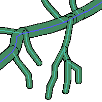 |
Dissolve
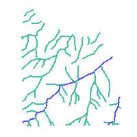
We are going to generate a new table "dis1" with the resulting dissolution of the table "buf2"
create table dis1 (gid serial PRIMARY KEY);

--PostgreSQL
select addgeometrycolumn ('','dis1','geom',-1,'MULTIPOLYGON',2);
insert into dis1 (geom) select ST_Union (b.geom) from buf2 b;

--H2
select addgeometrycolumn ('','DIS1','GEOM',-1,'MULTIPOLYGON',2);
insert into dis1 (geom) select ST_UnionAgg (b.geom) from buf2 b;
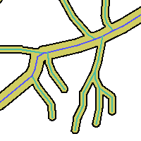 |
Dissolve boundaries by Attribute
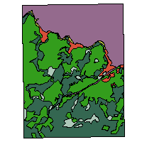
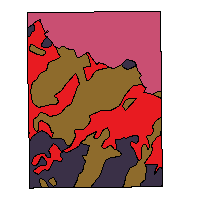
Now, we are going to dissolve boundaries in the table "soils" by the attribute "soil_code". The result is stored in the table "dis2"
CREATE TABLE dis2 (gid serial PRIMARY KEY, soil_code integer);

--PostgreSQL
SELECT addgeometrycolumn ('','dis2','geom',-1 ,'MULTIPOLYGON',2);
INSERT INTO dis2 (geom,soil_code) SELECT ST_Multi(ST_Union (s1.geom)), s1.soil_code
  FROM soils AS s1
  GROUP BY s1.soil_code;

--H2
SELECT addgeometrycolumn ('','DIS2','GEOM',-1 ,'MULTIPOLYGON',2);
INSERT INTO dis2 (geom,soil_code) SELECT ST_Multi(ST_UnionAgg (s1.geom)), s1.soil_code
  FROM soils AS s1
  GROUP BY s1.soil_code;

SELECT ST_GeometryType(geom) as typeGeom, count(*) as num
 FROM dis2 group by typeGeom;

    typegeom     | num
-----------------+-----
 ST_MultiPolygon |   4
(1 row)
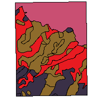 |  |
You can obtain the same result of the dissolution using ST_Collect with ST_Dump. ST_Collect will return a MULTI geom from the single geometries obtained with ST_Dump
--PostgreSQL
CREATE TABLE dis3 (gid serial PRIMARY KEY,soil_code integer);

--PostgreSQL
SELECT addgeometrycolumn ('','dis3','geom',-1 ,'MULTIPOLYGON',2);
INSERT INTO dis3(soil_code,geom) SELECT soil_code, (ST_Multi(ST_Collect(foo.the_geom))) as geom
 FROM (SELECT soil_code, (ST_Dump(geom)) As the_geom FROM soils) As foo GROUP BY soil_code;

--H2
SELECT addgeometrycolumn ('','DIS3','GEOM',-1 ,'MULTIPOLYGON',2);
INSERT INTO dis3(soil_code,geom) SELECT soil_code, ST_Multi(ST_Collectagg(geom))
FROM dump('SELECT geom as geom, soil_code as soil_code FROM soils') As foo GROUP BY soil_code ; Obtain the polygons with use_code=300 that are within a distance of 200 meters to the buffer calculated before.
SELECT u.gid AS id, u.use_code, ST_Distance(u.geom, dis1.geom) AS distance
 FROM uses u, dis1
 WHERE (ST_DWithin(u.geom, dis1.geom,200) AND u.use_code=300)
 ORDER BY distance, id;

 id | use_code |     distance
----+----------+------------------
 19 |   300    |         0
 23 |   300    |         0
 29 |   300    |         0
 33 |   300    |         0
 37 |   300    |         0
 47 |   300    |         0
 49 |   300    |         0
 50 |   300    |         0
 54 |   300    |         0
 57 |   300    |         0
 58 |   300    |         0
 61 |   300    |         0
 64 |   300    |         0
 65 |   300    |         0
 71 |   300    |         0
 74 |   300    |         0
 66 |   300    | 1.89932166720597
 28 |   300    | 5.27330754254734
 24 |   300    | 12.9027980215524
 69 |   300    | 20.0068276577405
 56 |   300    | 37.0450602191106
 72 |   300    | 61.5356033535093
 34 |   300    | 69.8226892487313
 70 |   300    | 70.5942141324269
 40 |   300    | 90.4315260748462
 53 |   300    | 91.4044158396345
(26 rows)
Let's update a Spatial Reference System Identifier of the table "centroid_uses". You can check that the coordinates aren't re-projected.
--PostgreSQL
SELECT UpdateGeometrySrid('centroid_uses','geom',25830);
--H2
SELECT UpdateGeometrySrid('CENTROID_USES','GEOM',25830);


SELECT ST_AsEWKT(geom) FROM centroid_uses c ORDER BY c.id LIMIT 1;

                   st_asewkt
-----------------------------------------------
 SRID=25830;POINT (5311.9800000000005 6902.99)
(1 row)
If you want to re-project a geometry value you should use the ST_Transform function.
Re-projection
--PostgreSQL
SELECT UpdateGeometrySrid('centroid_uses','geom',4326);
--H2
SELECT UpdateGeometrySrid('CENTROID_USES','GEOM',4326);


UPDATE centroid_uses SET geom=(ST_Transform(ST_SetSRID(geom,25830),4326)) ;
SELECT ST_AsEWKT(geom) FROM centroid_uses c ORDER BY c.id LIMIT 1;

                       st_asewkt
--------------------------------------------------------
 SRID=4326;POINT (-7.441154927102713 0.062264726485138)
(1 row)